

Pressure Vessel Failure: Case-Study
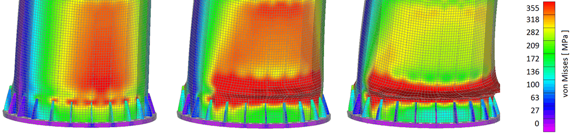
We were recently hired to investigate the cause of pressure vessel failure. In my line of work, I can…
18 February 2026I literally run this blog for posts like this one. Recently a friend challenged me to do something in Nastran. At a certain point, I realized that I know too little about nonlinear material types in NX Nastran and I suspect this is why I have convergence problems in my task. So as typical me, I stopped a challenge and decided to learn more about material nonlinearity, starting from the simplest models to the most advanced ones when it comes to steel 🙂
This will be described from NX Nastran standpoint, but those models are used in most FEA codes. If you are interested in the general version (not the NX Nastran specific) go here.
First of all, let’s go with the NX Nastran “Basic” nonlinear solver: SOL 106. It’s called “basic” since there is also an Advanced nonlinear solver (SOL 601) also known as Adina (I’m a big fan of Prof. Bathe’s work!). In SOL 106 Nastran give us several approaches to material nonlinearity:
Most common nonlinear material models:
This is the first type of material nonlinearity one can set in SOL 106. It is dedicated only to isotropic materials. The nonlinear elastic material will not yield, which means that however high the load will be, after taking that load away the material will return to its initial state without any permanent deformations. It also does not show strain hardening (after several times loading-unloading cycles it acts the same).
To define it you should make stress vs strain function (in Femap it is called Function Dependence). This function can be defined for the first and third quadrant (positive stress + positive strain and negative stress + negative strain) – this takes into account that material may exhibit different properties in compression. If you define the function only in the first quadrant the first point must be at 0.0 point. It will be assumed that the relation in tension and compression are the same. If you are using Femap please note that you should use a chart 4.. vs Stress when you are defining the nonlinear property (there is also stress vs strain function).
For NX Nastran geeks 🙂
KEYWORD MATS1:
I’m tempted to write this is a “default” nonlinear material for steel. It is not as robust as the third option, but really easy to set up instead. This material can include strain hardening (also kinematic+isotropic hardening is an option). You can define this material in several ways. First of all, you need to define which yield criterion will be used – 4 possibilities are present:
Yield criterion described in field YF (Yield Function):
When you decide on the proper yield criterion (for steel von Misses is used), you need to input initial yield stress (for von Mises and Tresca) or 2*cohesion and angle of internal friction (for Mohr-Coulomb and Drucker – Prager). Then the work hardening slope has to be defined unless you want your material to be perfectly plastic (which is a default setting in NX Nastran and in Femap). Work hardening slope H (in units of stress) is a slope of stress vs plastic strain, as shown below:

If you will have cyclic loads in your analysis, defining the hardening rule is a good idea. Sol 106 foresee 3 possibilities to do that:
Hardening Rule described in field HR

Join my 2h FREE Live Event and learn all that you need to know to start using Nonlinear FEA as an Expert! I will talk about:
Also note, that NX Nastran Keyword MATS1 field TYPE is PLASTIC – for those of you that use Femap and do not want to go deep in NX Nastran, this is also relevant. Since the type will be the same, it will be important which parameters you define. For bilinear material described here, you should input work hardening slope H and for the nonlinear elastoplastic material you will implement the stress–strain curve. This means you should never define two at the same time.
For NX Nastran geeks 🙂
KEYWORD MATS1:
This is the more advanced option than the bilinear material described previously. A lot of settings remain the same (YF, HR, initial yield point). Instead of work hardening slope H, you have to define a curve showing a multi-linear relation between stress and strain. In Femap, this curve should be defined as 4.. vs Stress function. NX Nastran will interpret this curve as engineering stress (true stress-strain is not supported in SOL 106).
If you want to have true stress-strain this is possible in SOL 601. Parameter CSVSSVAL allows for recalculation of provided engineering stress-strain curve into a true stress-strain one. Femap allows this with an option “convert dependency to true stress” in the Advanced Nonlinear solver settings window.
The stress-strain curve for this type of material must be defined starting in (ε=0; σ=0) point. The second point on the curve should be at initial yield (ε1; σy) for von Mises and Tresca. For Mohr – Coulomb and Drucker – Prager models this second point should be (ε1; 2c). The slope of the line connecting those first 2 data points must equal the value of E given in Femap (MAT1 entry). Work hardening slope Hk for each following step is calculated as follows:
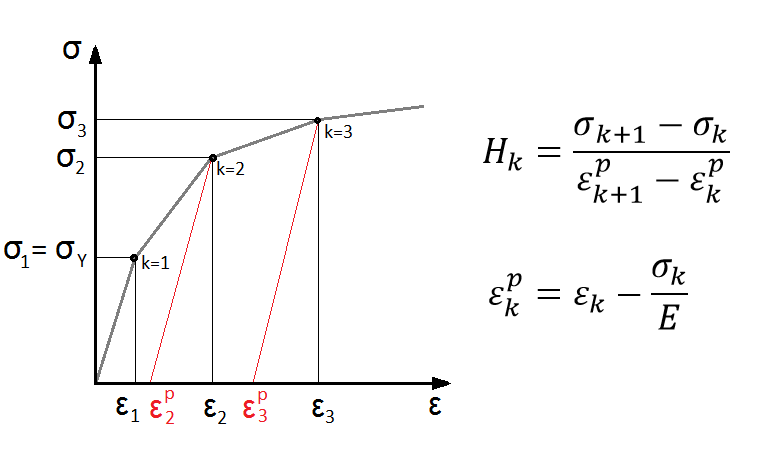
where  is the plastic strain in point k.
Note that you may provide the stress for initial yield not only by the curve above but also in the LIMIT1 field (in Femap the field is called Initial Yield Stress). If the value given in the chart does not match the value in this field, the value in the LIMIT1 field takes precedence when calculating strain at yield. However, the work hardening slope will be still calculated according to values in the chart as shown above.
Note that in NX Nastran isotropic plasticity theory is used to calculate plastic strains, regardless of the material type defined for an elastic range.
For NX Nastran geeks 🙂
KEYWORD MATS1:
I don’t think this material is used all too often, but since it is a possibility in MATS1 I decided to write something about it as well. Most of the settings are identical as for the previous 2 examples. Here, however, we are choosing TYPE = PLSTRN. This leads to a situation where we define only the plastic part of a stress-strain curve – the solver will assume that material is rigid in the elastic regime. I think that the graph below clearly shows everything:

Settings and parameters I mentioned above are dedicated to SOL 106. Most of them work in SOL 601 as well with some additional requirements:
Selected additional Sol 601 requirements:
Hey! Thanks for reading. I usually do not ask for comments but if you enjoyed it / found it useful leave a mark below in the comments – I would love to know how many other NX Nastran geeks are out there!
You can also read this awesome post by Blas Molero Hidalgo from Iberisa!



Share
Join the discussion